A team ships a 70B model behind an API, watches the GPU bill land at $2,000 to $3,000 a day, and concludes that inference is just expensive. Then someone checks utilization and finds that the fleet is sized for peak concurrency while most of the GPUs spend most of their time streaming weights out of memory to produce one token for one user.
A 70B model at FP16 needs about 140GB just for weights, so a single replica is two A100 80GBs at minimum and four in practice once you leave room for the KV cache. At $3 to $4 per GPU-hour that is roughly $300 to $400 a day for one replica. Five to ten replicas, which is 20 to 40 A100s and a real deployment rather than a pilot, puts you at $2,000 to $3,000 per day. That is $60K to $90K per month for one model. Add a second model and a second region and the number stops being a line item and starts being a conversation with finance.
The useful thing about that bill is how much of it is recoverable. Cutting it by 40 to 60 percent without measurably hurting output quality is normal, not clever. The reason it is normal is that most serving stacks are configured as if inference were one kind of work, when it is actually two kinds of work with opposite bottlenecks.
Prefill and decode are different machines
Every request you serve has two phases, and almost every costly mistake comes from treating them as one.
Prefill processes the prompt. All the input tokens go through the model at once, in parallel, as one big matrix multiply. It is compute-bound. The GPU's arithmetic units are the constraint, and a long prompt saturates them nicely.
Decode generates the output, one token at a time. Each new token requires reading the entire set of model weights out of memory to produce a single token. It is memory-bandwidth-bound. The arithmetic is trivial and the bus is the constraint.
That asymmetry is the whole game. In decode, you are paying to stream gigabytes of weights from HBM to compute one token for one user. If a second user is mid-generation at the same moment, their token rides along on the same weight read at nearly zero marginal cost. This is why batching is not a modest optimization. It is the difference between paying for weight reads per user and amortizing them across everyone.
It also explains why the two phases want different service level objectives. Prefill determines time to first token. Decode determines time per output token, which the user experiences as how fast the text streams. Averaging them into one latency number hides the tradeoff you are about to make.
Where the cost actually goes
Four places, in rough order of how much money is usually sitting in them.
GPU hours. The headline number, and the one everyone tries to cut by asking for a discount rather than by raising occupancy.
Memory bandwidth. Not a line on the invoice, which is why it gets missed. You pay for it as GPU hours that produce very few tokens.
Idle time. GPUs held warm and waiting. Cheap to ignore, expensive to accumulate, and invisible unless you track utilization rather than request count.
Network egress. Usually small for text, and worth checking anyway if you are shipping long contexts across regions or pulling multi-gigabyte weights on every cold start.
Four levers, in the order I pull them
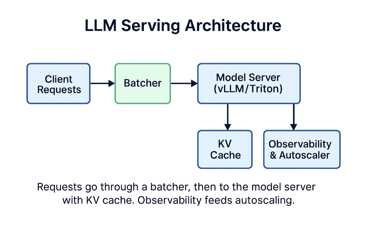
1. Batch continuously, not statically
Combine requests so one pass through the weights serves many users. Throughput improvement of 2x to 4x is the normal result, which means fewer GPUs for the same load.
The important distinction is static versus continuous batching. Static batching collects a fixed group of requests, runs them together, and waits for all of them to finish before starting the next group. One request generating 800 tokens holds the whole batch hostage while a request that needed 20 tokens sits there finished, occupying a slot.
Continuous batching schedules at the granularity of a single decode step instead of a whole request. It evicts each sequence the moment it emits its stop token and admits a new request into that slot on the next step. Orca introduced this iteration-level scheduling in 2022; vLLM is where most people met it, and its own contribution is the paged memory management underneath. The batch composition changes every iteration. On mixed output lengths, which is every real workload, this is where most of the throughput comes from.
The cost is latency at low traffic. If requests arrive slowly and you wait to fill a batch, you are adding queue time to serve nobody. Set a maximum wait of 10 to 20 milliseconds and let the batch go early when it expires. Under load the window never fires because the batch fills first.
Long prompts cause the other failure here. A single 30,000 token prefill monopolizes the GPU for hundreds of milliseconds, and every user already streaming tokens stalls behind it. Chunked prefill splits that work into pieces and interleaves them with decode steps, so one large prompt stops being a latency event for everyone else.
2. Reuse the KV cache, and know what it costs you
The cache holds the key and value tensors for tokens already processed, so you are not recomputing attention over the whole prefix on every step. Framing this as a percentage saving undersells it. Generating N tokens without a cache reprocesses on the order of N-squared token positions instead of N, which at a few thousand tokens is a factor of a thousand, not a third. Nobody ships an uncached decoder. The cache is what makes autoregressive decode tractable at all, so the engineering question is never whether to use it, only what it costs you.
What gets underestimated is the memory. Cache size scales with batch size times sequence length times layers times key-value heads times head dimension times bytes per element, twice over for keys and values. At long context and high concurrency it stops being a detail and becomes the thing that decides your maximum batch size, which means it decides your throughput, which means it decides your bill.
Three things follow from that. Attention variants that share key-value heads across query heads shrink the cache by exactly the ratio between them. Llama-2-70B has 64 query heads and 8 key-value heads, so grouped-query attention cuts the cache 8x; multi-query attention at a single key-value head would be 64x. This is a property of the model you picked rather than something you can tune at serving time, which is why it belongs in the model selection conversation. Paged allocation, the idea behind PagedAttention, stores the cache in fixed blocks instead of one contiguous reservation per sequence, which removes the fragmentation that otherwise wastes a good fraction of your memory. And quantizing the cache itself to 8 bits buys back room for more concurrent sequences.
The highest-return case is prefix caching. If every request begins with the same 2,000 token system prompt, you are paying to prefill identical tokens on every single call. Cache that prefix once and reuse it across requests. For agent workloads and long few-shot prompts, this alone can remove most of your prefill cost.
Long-lived sessions need an eviction policy. Without one the cache grows until allocation fails, and the failure shows up as throughput collapse rather than an obvious error.
3. Quantize the weights, then verify on your own evals
Lower precision weights mean less memory to move, and since decode is bandwidth-bound, less memory to move means more tokens per second. INT4 cuts weight memory by roughly 75 percent against FP16. It does nothing for the KV cache or activations, so at long context and high concurrency your actual footprint drops by much less than that, sometimes by very little. Published kernel benchmarks for AWQ and GPTQ report 3x and better; in a batched server where you were already amortizing weight reads across a batch, expect 1.5x to 2x end to end. FP8 on newer hardware gives a smaller gain with less quality risk.
Weight-only quantization, which is what AWQ and GPTQ do, is the conservative starting point. Weights are stored at 4 bits and dequantized for compute, so activations stay at higher precision and the damage is limited. Quantizing activations too goes further and is a real quality decision.
Here is the part that gets skipped. Aggregate benchmark scores are close to useless for deciding whether a quantized model is safe to ship. Perplexity barely moves while the specific behavior you depend on degrades. Quantization tends to hurt the long tail first: rare formats, structured output, arithmetic, low-resource languages, instruction following at the edges. If your product is JSON-emitting tool calls, measure JSON validity and tool-call accuracy, not perplexity. Run it on your own golden set before it reaches a user.
4. Schedule for occupancy
Once the first three are in place, scheduling is worth another 10 to 20 percent on top.
Keep a small warm pool so requests are not paying for cold starts, because loading tens of gigabytes of weights is a slow, visible stall. Scale on a signal that reflects the actual constraint, which is queue depth or batch occupancy, not CPU. Bin-pack smaller models onto shared GPUs instead of giving each one a dedicated device it cannot fill.
Then check whether you are running on the right hardware at all. The reflex is to reach for the largest available accelerator, but a smaller GPU with enough memory to hold the model often wins on cost per token because it is cheaper per hour and you were bandwidth-bound anyway. The metric that matters is cost per million tokens at your latency target, not raw peak throughput.
Both directions here have a failure mode. Over-scaling erases the savings you just made. Under-scaling shows up as cold starts and queue time during the traffic spike you built all of this for.
The trade-offs, stated plainly
Batching against latency. Excellent for throughput, adds wait time. Bounded by the maximum wait you configure.
Quantization against quality. INT4 saves real money and can hurt accuracy in ways aggregate metrics do not surface.
KV cache against memory. Faster inference, and the cache competes with batch size for the same memory. Sometimes a smaller cache and a larger batch is the cheaper configuration.
Autoscaling against stability. Aggressive scaling saves money and causes cold starts.
The number that reconciles these is not throughput. It is goodput: requests per second that actually met your latency target. A stack tuned for peak throughput will happily report a large number while missing its time-to-first-token objective on a third of requests. Tokens per second that nobody accepted are not savings.
What I would do first
In order, because each step tells you whether the next one is worth doing.
Measure before changing anything. GPU utilization, batch occupancy, time to first token and time per output token at p95, and cost per million tokens. Without these you cannot tell a real improvement from a shifted bottleneck.
Turn on continuous batching with a bounded wait window. Enable paged KV cache and prefix caching, and confirm the cache is actually hitting rather than silently missing on a prompt that varies at the start. Test INT4 or FP8 against your own golden set and look at the tail behavior, not the average. Add autoscaling on queue depth with a warm pool. Then recheck cost per million tokens and see which constraint moved.
Batching and quantization together are where most of the money is. On a serving stack that started out unoptimized, the two of them account for the bulk of a 40 to 60 percent reduction.
Where this stops working
These techniques assume you are bandwidth-bound in decode and that you have enough concurrent traffic to fill a batch. Two situations break that assumption.
Very low traffic is the first. If you serve a handful of requests an hour, there is nothing to batch and nothing to amortize, and you are paying for a warm GPU to sit idle. Serverless or a shared endpoint is the honest answer, and the fix is architectural rather than a tuning parameter.
Strict latency floors are the second. If you need time to first token under 100 milliseconds at p99, every lever above trades against you, because they all buy throughput with queueing. That case is usually solved by routing: a small model handles most traffic and escalates to the large one only when it needs to. Which raises the question worth asking before any of this, namely whether the 70B model is required for the majority of your requests, or only for the ones you had in mind when you picked it.
References
Orca (OSDI 2022), for iteration-level scheduling
vLLM and the PagedAttention paper, for paged KV cache and prefix caching
Sarathi-Serve, for chunked prefill and the goodput framing
NVIDIA Triton Inference Server and TensorRT-LLM
AWQ and GPTQ for weight-only quantization
Subscribe for weekly AI infra deep dives.